Abstract
Abstract
We continuously detect sensory data, like sights and sounds, and use this information to guide our behaviour. However, rather than relying on single sensory channels, which are noisy and can be ambiguous alone, we merge information across our senses and leverage this combined signal. In biological networks, this process (multisensory integration) is implemented by multimodal neurons which are often thought to receive the information accumulated by unimodal areas, and to fuse this across channels; an algorithm we term accumulate-then-fuse. However, it remains an open question how well this theory generalises beyond the classical tasks used to test multimodal integration. Here, we explore this by developing novel multimodal tasks and deploying probabilistic, artificial and spiking neural network models. Using these models we demonstrate that multimodal units are not necessary for accuracy or balancing speed/accuracy in classical multimodal tasks, but are critical in a novel set of tasks in which we comodulate signals across channels. We show that these comodulation tasks require multimodal units to implement an alternative fuse-then-accumulate algorithm, which excels in naturalistic settings and is optimal for a wide class of multimodal problems. Finally, we link our findings to experimental results at multiple levels; from single neurons to behaviour. Ultimately, our work suggests that multimodal neurons may fuse-then-accumulate evidence across channels, and provides novel tasks and models for exploring this in biological systems.
* Joint-last authors
1Introduction
Animals are equipped with multiple sensory channels, each of which bears rich information about their environment. To maximise survival, this sensory data must be transformed into behavioural outputs Barlow, 1961. However, each channel is inherently noisy and can be ambiguous alone. For example, using just vision, it would be difficult to determine if an object was metal or a plastic imitation. As such, combining information across channels (multimodal integration) is advantageous as it reduces noise and ambiguity, and enables faster and more accurate decision making Trommershauser et al., 2011
The computational goal Marr, 1982 of multimodal integration is to infer the cause of sensory inputs; whether that be distinguishing self vs external motion from visual and vestibular cues Fetsch et al., 2012 or detecting prey in an environment cluttered with distracting sights and sounds. In biological networks, these computations are implemented by multimodal neurons, which receive inputs from multiple sensory channels and project to downstream areas. However, how to best describe these network’s input-output transformations, which we will term algorithms Marr & Poggio, 1976, remains an open question. One theory, the multisensory correlation detector Parise & Ernst, 2016, suggests that multimodal neurons receive temporally filtered information from each sensory channel and then compute the correlation and lag between channels. In contrast, the canonical view suggests that they receive the information separately accumulated by unimodal areas, linearly fuse this across channels, and then signal to decision outputs Fetsch et al., 2013 - an algorithm we term accumulate-then-fuse (AtF).
Support for this algorithm comes from work based on a set of classical multisensory tasks in which observers are presented with directional information in two channels, such as moving bars and lateralised sounds, and are trained to report the direction with the most evidence. In these tasks both the behaviour of observers Jones, 2016 and the activity of multimodal neurons Coen et al., 2023 are well described by the accumulate-then-fuse algorithm. Moreover, this algorithm is optimal in the sense that it generates unbiased (i.e., correct on average) estimates with minimum variance Trommershauser et al., 2011.
However, there are two open questions regarding the accumulate-then-fuse algorithm. First, the extent to which it generalises beyond the classical tasks used to explore multimodal integration Jones, 2016. Second, its relevance outside of a laboratory context. Indeed, while mice can be trained to use this algorithm, neither the behaviour nor neural activity of untrained mice are well described by it Coen et al., 2023.
Here, we explore the algorithms that multimodal neurons implement by developing novel multimodal tasks which focus on the underlying statistical relationships between channels rather than the details of the sensory signals themselves. This choice confers three major benefits. First, it allows us to design tasks which emphasise the importance of learning joint statistics across channels (like the natural relation between lip movements and speech). Second, it enables us to explore multimodal integration at three levels of abstraction: probabilistic ideal observers, minimal artificial neural networks and spiking neural networks trained via surrogate gradient descent Zenke & Ganguli, 2018. Third, by remaining agnostic to the specific stimuli, our tasks can easily be translated across experimental setups and model systems. Our results lead us to propose a new fuse-then-accumulate (FtA) algorithm for multimodal processing, which generalises and outperforms the canonical (AtF) algorithm and is optimal for a wide-class of multimodal problems.
2Results
2.1Multimodal units are not necessary for accuracy or balancing speed/accuracy in classical tasks
We began by training spiking neural networks to perform classical multisensory tasks. In these tasks we present sequences of directional information (left / right) in two channels, and train networks to report the direction of overall motion (Figure 1.B1). In a reduced case both channels always signal the same direction, while in an extended version we include both unimodal and conflicting trials. Each network was composed of two unimodal areas with feedforward connections to a multimodal layer, connected to two linear output units representing left and right choices (Figure 1.A1). Following training, multimodal networks achieved a mean test accuracy of 93.4% (±0.1% std) on the reduced task and 94.2% (±0.05% std) on the extended task. In line with experimental work Coen et al., 2023 their accuracy on the extended task varied by trial type (Supplementary Fig.1).
To understand the role multimodal units play in these tasks, we trained two additional sets of networks: one without a multisensory layer (Figure 1.A2) and, to control for network depth, one in which we substituted the multisensory layer for two additional unimodal areas (Figure 1.A3). Surprisingly, these architectures performed similarly to the multimodal architecture on both the reduced (unimodal: 93.9%, ±0.2% std; 2-unimodal: 93.0%, ±0.2% std) and extended task (unimodal: 94.1%, ±0.1% std; 2-unimodal: 94.1%, ±0.1% std), suggesting that multimodal spiking units are not necessary for accuracy on these tasks. So, what computational role do these units play? One alternative is that they are beneficial in balancing speed/accuracy Drugowitsch et al., 2014. However, we found that all three architectures accumulated evidence at equivalent rates (Figure 1.C1).
While these results may seem surprising, the optimal strategy in this task simply amounts to accumulating each channel’s evidence separately, and then linearly fusing this information across channels to form a final estimate. In our models, this accumulate-then-fuse (AtF) algorithm (Figure 1.D) can be directly implemented by the output units, as it is a linear computation, and consequently, an intermediate multisensory layer provides no benefit. Beyond our models, these results raise the question of when or why biological networks would require multisensory neurons between their unimodal inputs and downstream outputs.

Figure 1:A1-3 Network architectures - spikes flow forward from input channels (Ch0, Ch1) to decision outputs (D). B1-2 Tasks are sequences of discrete symbols (left, neutral, right) per channel, with a fixed number of time steps, and a label (left or right). In classical tasks (B1) this label indicates the overall bias (e.g. L > R). In comodulation tasks (B2) this label is encoded jointly across channels (e.g. LL > RR). **C1-2**Test accuracy as a function of time for the reduced classical (C1) and probabilistic comodulation (C2) tasks. We plot the mean (line) and standard deviation (shaded surround) across 5 networks per architecture, plus the optimal accuracy from the FtA algorithm (grey line). D In classical tasks the optimal algorithm is to accumulate-then-fuse evidence across channels. E In comodulation tasks fuse-then-accumulate is optimal.
2.2Multimodal units are critical for extracting comodulated information
To explore when networks need multisensory neurons, we designed a novel task in which we comodulate signals from two channels to generate trials with two properties (Figure 1.B2):
- Within each channel there are an equal number of left and right observations, so a single channel considered in isolation carries no information about the correct global direction.
- On a fraction of randomly selected time steps (which we term the joint signal strength), both channels are set to indicate the correct direction. Then the remaining observations are shuffled randomly between the remaining time steps (respecting property 1). Thus each trials label is encoded jointly across channels.
As above, we trained and tested all three architectures on this task. Strikingly, both unimodal architectures remained at chance accuracy (unimodal: 50.4%, ±0.4% std; 2-unimodal: 50.4%, ±0.3% std), while multimodal networks learned the task well (multimodal: 96.0%, ±1.3% std). Additionally, multimodal network accuracy increased in line with joint signal strength (Supplementary Fig.2). However, this task seems unrealistic – as it requires a perfect balance between labels – so we developed a probabilistic version with the same constraint (i.e., information is balanced on average but may vary on any individual trial). Again, both unimodal architectures remained at chance accuracy, while multimodal networks approached ideal performance (Figure 1.C2).
Together, these results demonstrate that multimodal units are critical for comodulation tasks, though why is this the case? In contrast to classical multisensory tasks, our comodulation tasks require observers to detect coincidences between channels and to assign more evidential weight to these than non-coincident time points. As such, observers must fuse information across channels before evidence accumulation; an algorithm which we term fuse-then-accumulate (FtA) (Figure 1.E). In our unimodal architectures, fusion happens only at the decision outputs which are linear, meaning they are unable to assign coincidence a higher weight than the sum of the individual observations from each channel. Consequently, the algorithm they implement is equivalent to accumulate-then-fuse. In contrast, our multimodal, leaky integrate-and-fire, units can assign variable weight to coincidence via their nonlinear input-output function.
2.3The fuse-then-accumulate algorithm excels in naturalistic settings
Our results demonstrate that the fuse-then-accumulate algorithm can solve comodulation tasks where accumulate-then-fuse remains at chance level, but would these two algorithms differ in naturalistic settings? To explore this, we adapted the tasks above to produce a novel detection task in which a predator must use signals from two channels, e.g., vision and hearing, to determine both whether prey are present and if so their direction of motion (3-way classification). In this task, trials are generated via a probabilistic model with 5 parameters which specify the probability of: prey being present in a given trial (), emitting cues at a given time when present (), signalling their correct () or incorrect () direction of motion and the level of background cues () (Figure 2.A-B). This task thus closely resembles those above in structure, but with the added realism that information arrives at sparse, unspecified intervals through time.
Using this task, we first compared how the accuracy of the two algorithms differed in distinct settings. To do so, we randomly sampled 10,000 combinations of the 5 task parameters and used ideal Bayesian models to determine each algorithm's accuracy. To meaningfully compare the two algorithms we then filtered these results to keep those above chance but below ceiling accuracy. This process left us with 2,836 (28%) sets of parameter combinations. Across these settings, FtA always performs better than AtF, and the median difference (FtA minus AtF) was 0.73%. Though, the maximum difference was 13.7%, showing that while FtA is always as good as AtF, it excels in specific settings.
To understand when FtA excels compared to AtF, we calculated each parameter's correlation with the difference in accuracy and it's importance in predicting it using a random forest regression model (Section 4.6.2) (Figure 2.C-D). This approach revealed that FtA excels when prey signal their direction of motion more reliably (increasing ), but more sparsely in time (decreasing ). Critically, these settings resemble naturalistic conditions in which prey provide reliable cues, but try to minimise their availability to predators by remaining as concealed as possible.
Next, we focused on a subset of detection settings by fixing , and and identifying combinations of and where FtA consistently achieves 80% accuracy. Across this subset, AtF’s accuracy decreases with the sparsity of the signal, a function of and (Figure 2.E). Finally, we trained spiking neural networks on the two extremes of this subset: one in which prey emit unreliable signals, densely in time (dense detection) and one in which prey emit reliable signals, sparsely in time (sparse detection). In the dense setting, we found no difference in either accuracy or reaction time between the three architectures (Figure 2.F). In contrast, the multimodal architecture outperformed both unimodal architectures in the sparse setting (Figure 2.G).
Together these results demonstrate that the FtA algorithm is always as good as AtF, but excels in naturalistic settings when prey emit reliable signals, sparsely in time.

Figure 2:A-B In the detection task, a 5 parameter probabilistic model generates trials (sequences of discrete symbols) with different statistics. At each time step there is either a signal emitted ( with probability if there is a prey present) or not () with different probability distributions depending on the value of . C Each parameter’s importance (bars) in predicting the difference in accuracy between the ideal FtA and AtF models, as determined by a random forest regression model, and each parameters correlation with the difference (arrows). D The difference in accuracy between the two algorithms as a function of the tasks 5 parameters. For each detection setting (a set of 5 parameters values), we plot the value of each parameter (subplots) and the difference between the two algorithms across 10,000 trials. Overlaid (coral lines) are linear regressors per parameter. The rightmost subplot shows a kernel density estimate of the difference across detection settings. E The accuracy of each ideal algorithm across a subset of detection settings where we vary the signal sparsity - a function of pe and pc. F-G The test accuracy over time of our three SNN architectures, plus the optimal accuracy from the FtA algorithm (grey line), on the two extremes of the family in E.
2.4The softplus nonlinearity solves a wide class of multimodal problems
Above, we have focused on tasks in which observers must use information from two sensory channels to reach one of two or three possible decisions. However, even the simplest of organisms are granted more senses and possible behaviours. Thus, we now compare the accumulate-then-fuse and fuse-then-accumulate algorithms in more generalised settings. To do so, we consider the more general case of channels and directions (or classes, more generally).
In the most general case, solving this task would require learning the joint distribution of all variables, i.e. parameters, which would quickly become infeasible as and increase. However, when channels are independent given a shared (underlying time dependent) variable, as in our detection task, it turns out that the optimal solution requires only a small increase in the number of parameters (a fraction more parameters) and a single nonlinearity (the softplus function) to the classical linear model (Figure 3.A and details in Section 4.1.6 and Section 7.3.3).
So, where does this softplus nonlinearity come from? For the isotropic case (for simplicity), following our derivation (Section 7.3.3) we arrive at the equation:
where is the direction being estimated, and is the number of the channels at time that indicate direction (that can take any value between and ). Our observer then estimates by computing at each time via a linear summation across channels, passing it through the nonlinear softplus function (), summing these values linearly over time to get the log odds of each possible direction and then estimating to be the value of which gives the maximum value (Figure 3.A). This provides us with two insights:
- As the number of channels () increases, the function gets closer to a shifted rectified linear unit (ReLU). That is, it gets close to returning the value 0 when is less than some threshold (), and afterwards is proportional to . Consequently, with many channels, the optimal algorithm should ignore time windows () where the evidence is below a certain threshold , and linearly weight those above (Figure 3.B).
- As the input becomes more dense, in our case as approaches 1, the optimal algorithm becomes entirely linear. As such, we can see why classical multisensory studies, which have focused on dense tasks, concluded that the linear AtF algorithm was optimal (Figure 3.B).
Returning to our ideal observer models, in these extended settings we found that the difference between the two algorithms (FtA minus AtF) increases with both the number of directions () and channels () (Figure 3.C). As above (Section 2.3), we observe little difference in dense settings (Figure 3.D) but large differences, up to 30% improvements of FtA over AtF, in sparse settings (Figure 3.E).
Finally, we adapted the observations in this multi-direction, multi-channel task, from discrete to continuous values with any probability distribution (Section 4.1.7) and show results for the Gaussian case. Mathematically, the optimal algorithm in the Gaussian case has the form . While this demonstrates that the exact form of the optimal function will depend upon the distribution of each channel’s signals; it suggests the softplus function will suit a wide class of multimodal problems. Extending our ideal observer models to this continuous case, generated similar results to the discrete case. That is, the difference between the two algorithms was negligible in dense, but large in sparse, settings (Supplementary Fig.3).
Together, these results explain why prior studies have focused on AtF, and demonstrate how just a small increase in algorithmic complexity (from AtF to FtA) leads to large improvements in performance across a wide class of multimodal problems.

Figure 3:A In the case of NC(channels) and ND(directions) the optimal algorithm is to sum the evidence for each direction across channels, apply a non-linearity () and then accumulate these values. B The optimal nonlinearity depends on both the number of channels which indicate the same direction () and the sparsity of the signal (pe). C The difference between the two algorithms depends on both the number of channels and directions. D-E Accuracy over time curves for the AtF (blue) and FtA (coral) algorithms in dense (D) and sparse (E) settings with 5 channels and 6 directions.
2.5Network implementations of FtA
Above, we demonstrated that the softplus nonlinearity is the optimal algorithm for a wide class of multimodal problems. Here, in the vein of Marr’s hardware level Marr, 1982Marr & Poggio, 1976, we explore how networks can implement this algorithm and how one can distinguish which algorithm (AtF or FtA) an observer’s behaviour more closely resembles.
2.5.1Network behaviour is robust across nonlinearities
To explore how precisely networks need to approximate the softplus function (or if any nonlinearity will do) we trained minimal artificial neural networks on our two channel tasks, and compared networks whose multimodal units used linear, rectified linear, sigmoidal or softplus activation functions (Section 4.3). In tasks with little comodulation (classical and dense-detection), linear activations were sufficient (Figure 4.A). In contrast, tasks with more comodulation (sparse-detection and comod) required non-linear activations, though all three non-linearities were equivalent in terms of both accuracy and reaction speeds (Supplementary Fig.4); suggesting that any non-linear function may be sufficient. Though, how do these mathematical functions relate to the activity patterns of real spiking neurons?
2.5.2Simple, single neuron models generate sub- to super-additive states
In experimental studies Stanford et al., 2005 the input-output functions of individual multimodal neurons are often inferred by comparing their multimodal response () to the sum of their unimodal responses () via a metric known as additivity:
Using this metric, neurons can be characterised as being in sub- or super-additive states (i.e., outputting less or more spikes than expected based on their unimodal responses) Stanford et al., 2005. However, the link between these neuron states and network behaviour remains unclear Jones, 2016. To explore this we conducted two experiments; one at a single neuron level (here) and one at the network level (Section 2.5.3).
To understand how these states arise in spiking neurons, we simulated single multimodal units, with differing membrane time constants () and mean input weights (), and calculated their additivity as we varied the mean firing rates of their input units () (Figure 4.B). These simulations recapitulated two experimental results, and yielded two novel insights. In agreement with experimental data Stanford et al., 2005 most units (60%) exhibited multiple states, and we found that lower input levels (both weights and firing rates) led to higher additivity values (Figure 4.B); a phenomenon termed inverse effectiveness Fetsch et al., 2013. Moving beyond experimental data, our simple, feedforward model generated all states, from sub- to super-additive; suggesting that other proposed mechanisms, such as divisive normalisation Ohshiro et al. (2011), may be unnecessary in this context. Further, we found that units with shorter membrane time constants, i.e. faster decay, were associated with higher additivity values (Figure 4.B); suggesting that this may be an interesting feature to characterise in real multimodal circuits. Notably, an alternative modelling approach (Section 4.4.2), in which we approximated the firing rates of single multimodal neurons Goodman et al., 2018Fourcaud & Brunel, 2002, generated almost identical results (Figure 4.B-right).
2.5.3Unit ablations demonstrate a causal link between additivity and network behaviour
To understand how these unit states relate to network behaviour we calculated the additivity of the multimodal units in our trained spiking neural networks, and compared these values across tasks. We found that most units were super-additive, though observed slight differences across tasks (Figure 4.C); suggesting a potential link between single unit additivity and network behaviour.
To test this link, we ranked units by their additivity (within each network), ablated the highest or lowest units and measured the resulting change in test accuracy. On the dense detection task, we found that ablating the units with lowest additivity had the greatest impact on performance, while on sparse detection we observed the opposite relation (Figure 4.D). The classical and probabilistic comodulation tasks respectively resembled the dense and sparse detection cases (Supplementary Fig.5). To understand these relations further we then ranked unit’s by their membrane time constants () or mean input weights () and repeated the -ablations. On both tasks ablating units with high input weights and / or long significantly impaired performance; highlighting the importance of accumulator-like units for both tasks. However, on sparse detection, we also observed that ablating units with short had a symmetrical effect (Figure 4.D); suggesting an additional role for coincidence-detector-like units on this task.
From these results, we draw two conclusions. First, different multimodal tasks require units with different properties (e.g. long vs short membrane time constants). Second, additivity can be used to identify the most important units in a network. However, as a unit’s additivity is a function of its intrinsic parameters (), additivity is best considered a proxy for these informative but harder to measure properties. Notably, an alternative approach in which we used combinatorial ablations (i.e. ablating unit 1, 1-2, 1-3 etc) to calculate each unit’s causal contribution to behaviour Fakhar & Hilgetag, 2022, yielded similar results (Supplementary Fig.6).
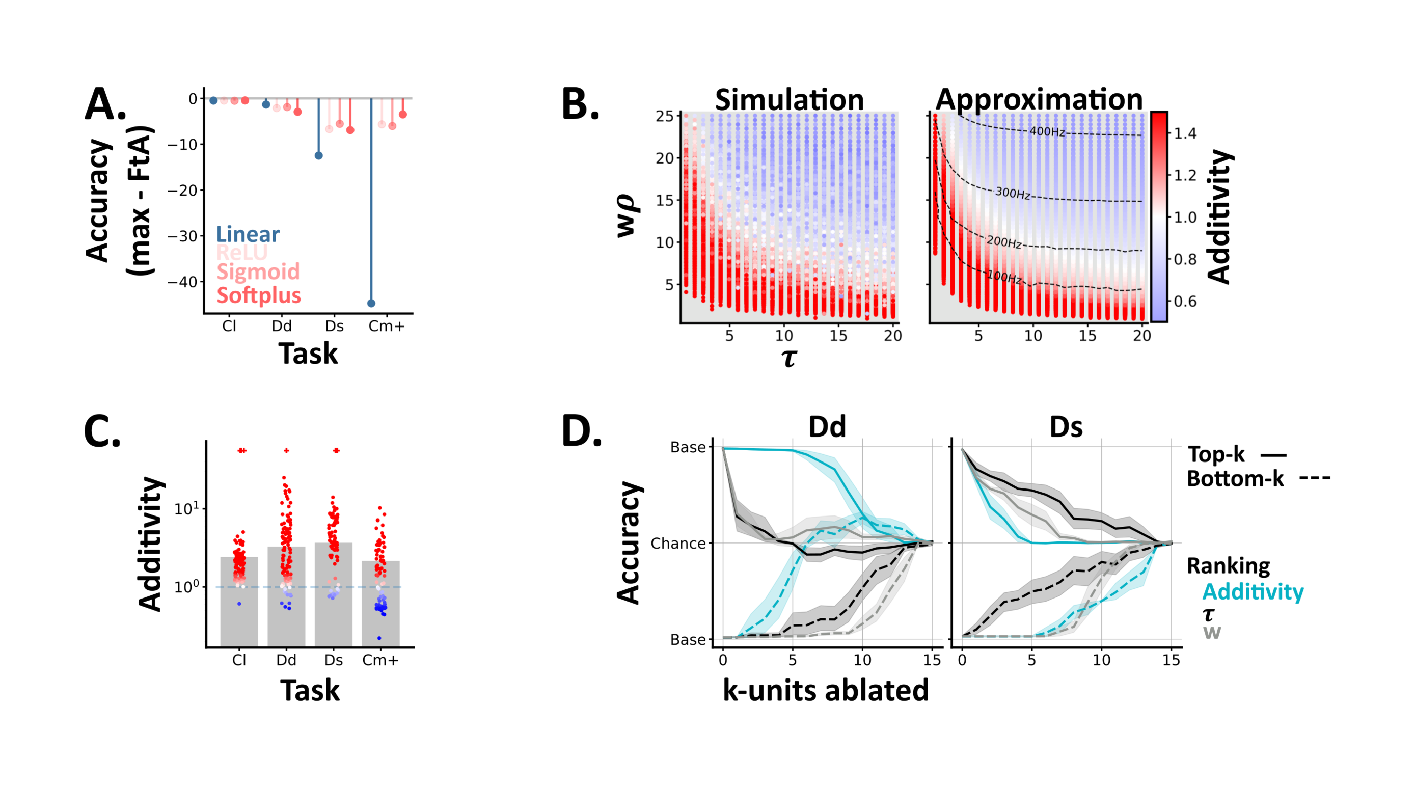
Figure 4:A ANN results. For each task (Cl: reduced classical, Dd: dense detection, Ds: sparse detection, Cm+: probabilistic comodulation) and activation function (colours) we plot the maximum test accuracy (across 5 networks) minus the optimal FtA accuracy. B Single unit model results. Each point shows the models additivity as a function of the membrane time constant (𝜏) and mean input (w⍴). The grey underlay shows when the multisensory unit fails to spike. The left panel shows the average additivity from 10 simulations. The right shows the results from an approximation method, with the multisensory unit’s firing rate (Hz) overlaid. C-D SNN results. C The additivity of each multisensory unit (circles) from spiking networks trained on different tasks. Bars indicate the mean additivity (across networks) per task. Colours, per unit, are as in B. Units which spike to multi-, but neither unisensory stimulus are denoted with a plus symbol. D Network accuracy, from baseline to chance, as we ablate either the top (solid lines) or bottom (dashed lines) k-units, ranked by different unit properties (colours). We plot the mean and std across networks, and invert the y-axis for the bottom-k results. Left / right - networks trained and tested on dense or sparse detection.
2.5.4Behaviour can distinguish which algorithm an observer is implementing
Finally, when testing an observer on a task, we wish to distinguish if their behaviour more closely resembles either algorithm (AtF or FtA). To do so, we measured the amount of evidence which each algorithm assigns to each direction (difference in log odds of direction left or right, given the observations), per trial, and then scattered these in a 2d space.
From this approach we garner two insights. First, by colouring each trial according to it’s ground truth label, we can visualise both the information available on each trial and the relations between tasks (Figure 5). For example, in the classical task both algorithms assign the same amount of evidence to each direction, so each trial lies along . In contrast, in the probabilistic comodulation task only FtA is able to extract any information, and all trials lie along the y-axis. Second, by colouring each trial according to an observers choices, we can compare how closely their behaviour resembles either algorithm (Figure 5). Applying this approach to our 2-layer unimodal, and multimodal SNN architectures illustrates that while their behaviour is indistinguishable on the classical and dense-detection tasks, there are a subset of sparse detection trials where the two algorithms choose opposite directions as their behaviour is respectively closer to the AtF or FtA algorithms (Figure 5).
Thus, coupled with task accuracy - which is all that is necessary on our comodulation tasks - trial-by-trial choices are sufficient to distinguish between the two algorithms.

Figure 5:For each subplot we scatter 2000 random trials on the same two axis: the amount of right minus left evidence according to each algorithm (Δ log odds). Thus, when x=0 the trial contains an equal amount of left and right information according to the AtF algorithm. Each column contains trials from a different task (Cl: reduced classical, Dd: dense detection, Ds: sparse detection, Cm+: probabilistic comodulation). The top row shows each trial’s label (left=blue, absent=off-white, right=orange). The middle and last row show the most common choice across 10 SNNs of either the 2-layered unimodal (middle) or multimodal (bottom) architecture. For these rows each trial’s alpha indicates how consistently networks chose the most common value. For example, on Cm+ the 2-unimodal networks choose randomly - and so these trials have a low alpha. Black arrows highlight subsets of trials where the two architectures choose opposite directions.
3Discussion
Prior experimental and theoretical work suggests that multimodal neurons receive the information accumulated by unimodal areas, and linearly fuse this across channels; an algorithm we term accumulate-then-fuse (AtF). In contrast, our results, from three levels of abstraction, suggest that they may fuse-then-accumulate (FtA) evidence across channels. Resolving which algorithm better describes multimodal processing in biological systems will require further experimental work. Nevertheless, here, we argue that FtA is likely to be a better description.
On classical tasks, both algorithms are indistinguishable and so describe multimodal processing equivalently. As such, prior experimental results are consistent with either algorithm. In contrast, on our novel comodulation tasks, AtF remains at chance level, while FtA is optimal. Thus, these tasks constitute simple experiments to determine which algorithm better describes an observer’s behaviour. However, both the classical and comodulation tasks seem unrealistic for two reasons. First, both are composed of dense signals (i.e. every time step is informative). Second, both treat the relations between channels in extreme ways: in the former, the temporal structure of the joint multimodal signal carries no information, while in the latter all the information is carried in the joint signal and the task is impossible using only one modality.
In contrast, in our detection-based tasks observers must extract periods of signal from background noise, and both the observations within and across channels are informative. As such, these tasks seems more plausible, particularly given the added realism that there is sometimes nothing to detect, and the fact that both algorithms can learn them to some extent. Moreover, unlike pure multisensory synchrony or coincidence detection tasks Parise & Ernst, 2016 in which the observer must explicitly detect coincidence, here coincidence is an informative, implicit feature. FtA is a generalisation of AtF and so always performs at least as well on our detection tasks. Though, FtA excels in realistic cases where prey signal their direction of motion reliably but sparsely in time, and in cases where the number of directions or channels is high. Note that while channels could originate from separate modalities, like vision or sound, our analysis also extends to independent sources of information from within modalities; so the number of channels may exceed the number of modalities. In sum, our results suggest that FtA could provide significant benefits in naturalistic settings and, assuming that performance is ecologically relevant, may constitute a better description of multimodal processing.
Though, there are three limitations to consider here. First, we focused on discrete stimulus tasks. Though, extending part of our work to the continuous case yielded similar results, and these tasks benefit from their interpretability Hyafil et al., 2023. Second, we focused on tasks with a fixed trial length. This is unnaturalistic as real tasks are temporally unbounded however, decoding observer’s accuracy over time hints at their performance in free-reaction tasks. Finally, we assumed that observations are generated by a single underlying cause. Relaxing this assumption and extending our work to consider causal inference is an exciting future direction Körding et al., 2007.
Beyond behaviour, are there hardware features which make either algorithm a better description of multimodal processing? In biological systems, these algorithms must be implemented by networks of spiking neurons, and each has specific requirements. In AtF, information is fused linearly across channels, and so every transformation in the network must be linear. In contrast, in FtA information should be fused nonlinearly via the softplus function. As neurons naturally transform their inputs via a spiking nonlinearity, and we show that the exact form of the nonlinearity is not critical, FtA constitutes a more natural solution for networks of spiking neurons. This argument is further supported by the that fact that the behaviour of trained SNNs more closely resembles FtA on both sparse-detection and comodulation tasks.
Ultimately, our work demonstrates that extending the AtF algorithm - with only a few additional parameters and a single nonlinearity - results in an algorithm (FtA) which is optimal for a wide class of multimodal problems; and may constitute a better description of multimodal processing in biological systems.
4Methods
In short, we introduced a family of related tasks (Section 4.1). In general, observers must infer a target motion (left or right) from a sequence of discrete observations in two or more channels – which each signal left, neutral or right at each time step. To approximate channels with equal reliability, we simply generated each channel's data using the same procedure. For each task we computed ideal performance using maximum a posteriori estimation (Section 4.2). When working with spiking neural networks we represented task signals via two populations of Poisson neurons per channel (Ch0) and (Ch1) with time-varying and signal-dependent firing rates (Section 4.5.1). In our spiking networks we modelled hidden units as leaky integrate-and-fire neurons (Section 4.4.1). Readout units were modelled using the same equation but were non-spiking. To ensure fair comparisons between architectures, we varied the number of units to match the number of trainable parameters as closely as possible. We trained networks using Adam Kingma & Ba, 2014, and in the backward pass replaced the derivative with the SuperSpike surrogate function Zenke & Ganguli, 2018. For all conditions we trained 5-10, networks, and report the mean and standard deviation across networks for each comparison.
4.1Tasks
For all tasks, there is a target motion to be inferred, represented by a discrete random variable . In addition, there is always a sequence of discrete time windows . At each time window , observations are made in each channel . In the case of two channels we will sometimes refer to and (evoking auditory and visual channels). Observations at different time windows will be assumed to be independent (except for the perfectly balanced comodulation task). For simplicity, we usually assume that information from each channel is equally reliable, and that each direction of target motion is equally likely, but these assumptions can be dropped without substantially changing our conclusions.
4.1.1Classical task
In the classical task we consider two channels, allow to take values representing left and right with equal probability, and assume that the channels are conditionally independent given . We define a family of tasks via a signal strength that gives the probability distribution of values of a given channel at a given time to be:
This has the properties that (a) when signal strength each value is equally likely () and the task is impossible, (b) as signal strength increases the chance of correct information increases and the chance of neutral or incorrect information decreases, (c) when signal strength all information is correct (, ). By default we use for this task.
4.1.2Extended classical task
In the extended classical task there are motion directions , for each channel ( with equal probabilities), along with signal strengths which both vary across trials. The overall motion direction is the direction of whichever modality has the higher signal strength in a given trial - we exclude trials when .
We also includes uni-sensory trials, when or . The probability distributions are the same as in (3) except with for and for .
4.1.3Perfectly balanced comodulation task
In the perfectly balanced comodulation task we use two channels and allow as in the classical task. We guarantee that in each channel, the number of left (-1), neutral (0) and right (+1) observations are precisely equal in number (one third of the total observations in each case). We define a signal strength and randomly select of the time windows in which we force . We set the remaining values of and randomly in such a way as to attain the per-channel balance in the number of observations of each value. Note that this is the only task in which observations in different time steps are not conditionally independent given .
4.1.4Probabilistically balanced comodulation task
The probabilistically balanced comodulation task is designed on the same principle as the perfectly balanced comodulation task but rather than enforcing a strict balance of left and right observations we only enforce an expected balance across trials, and this allows us to reintroduce the requirement that different time steps are independent. We define the notation where can take values (correct), (neutral) and (incorrect), and , and . We assume that the two channels are equivalent so and (to reduce the complexity) we assume since these cases carry no information about . The balance requirement gives us the equation or (by symmetry) . This gives us a two parameter family of tasks defined by these probabilities, and we choose a linear 1D family defined by a signal strength as follows:
This has the properties that when the task is impossible ( and ) and when the probability takes the highest possible value it can take (1/3). By default, we use for this task.
4.1.5Detection task
In the detection task we have two channels and now allow for the possibility where represents the absence of a target. We introduce an additional variable which represents whether the target is emitting a signal () or not (). If then for all , and if then is randomly assigned to 0 or 1 at each time step. When the probabilities of observing a left/right in any given channel are equal, whereas when you are more likely to observe a correct than incorrect value in a given channel. Channels are conditionally independent given and but dependent given only . We can summarise the probabilities as follows:
If we set the probability of a target being present and the emission probability then this reduces to the classical task.
We create a 1D family of detection tasks by first fixing (all values of equally likely), (all observations equally likely when signal not present), (signal reliable when present), and then picking from the smooth subset of values of and that give the ideal FtA model a performance level of 80%. We set for the point with the lowest value of and highest value of , and for the opposite extreme.
4.1.6Multichannel, multiclass detection task
We generalise the detection task to directions so and channels which can take any of these values, so for . We now assume there is always a target present and set . We make an isotropic assumption that every direction is equally likely (although see Section 7.3.3 for the non-isotropic calculations). In this case, when every observation is equally likely. When we let be the probability of a correct observation, and all other observations are equally likely. In summary:
4.1.7Continuous detection task
In the continuous detection task we allow the same set of values of as in the detection task, and the same definition of , but we now allow channels and each channel is a continuous variable that follows some probability distribution. For the general case, see the calculations in Section 7.3.4, but here we make the assumption that channels are normally distributed. If then and if then . By default we assume and , then vary and for the dense () and sparse () cases.
4.2Bayesian models
We define two maximum a posteriori (MAP) estimators for all tasks except the perfectly balanced comodulation task (because they assume that all time windows are conditionally independent given ). The estimator is:
Here is the vector of all observations . We give complete derivations in Section 7.3, but in summary this is equivalent to the following that we call the ideal fuse-then-accumulate (FTA) estimator:
If we additionally assume that channels are conditionally independent given (which is true for some tasks but not others) we get the classical estimator that we call accumulate-then-fuse:
We call this accumulate-then-fuse because each modality can accumulate the within-channel evidence separately before it is linearly fused across channels to get . In general, information from across channels needs to be nonlinearly combined at each time to compute before it is accumulated across time.
Note that when and are equally likely, this is akin to a classical drift-diffusion model. Let be the difference in evidence at time between right and left, . The decision variable given all the evidence up to time is which jumps in the positive direction when evidence in favour of motion right is received, and in the negative direction when evidence in favour of motion left is received. The estimator in this case is , i.e. right if the decision variables ends up positive, otherwise left.
In the classical task, this estimator simplifies to computing whether or not the number of times left is observed across all channels is greater than the number of times right is observed, and estimating left if so (or right otherwise). In the more general discrete cases you count the number of times each possible vector of observations across channels occurs and compute a weighted sum of these counts. In cases where it is not feasible to exactly compute the ideal weights, we can use a linear classifier using these vectors of counts as input, and we use this to approximate the AtF and FtA estimators for the perfectly balanced comodulation task.
4.3Artificial neural networks
Each minimal network was composed of: four unimodal units, two multimodal units and three decision outputs (prey-left, prey-absent or prey-right), connected via full, feedforward connections. Unimodal units were binary, and each sensitive to a single feature (e.g. channel 1 - left). Multimodal units transformed their weighted inputs via one of the following activation functions: linear, rectified linear (ReLU), sigmoid, or softplus of the form:
Where and are trainable parameters. To ensure fair comparisons across activations, we added two trainable biases to the other activations, such that all networks had a total of trainable parameters.
To read out a decision per trial, we summed the activity of each readout unit over time, and took the . To train networks, we initialised weights uniformly between 0 and 1, both and as 1, and used Adam Kingma & Ba, 2014 with: lr = 0.005, betas = (0.9, 0.999), and no weight decay.
4.4Single spiking neurons
4.4.1Simulation
We modelled each spiking unit as a leaky integrate-and-fire neuron with a resting potential of 0, a single membrane time constant , a threshold of 1 and a reset of 0. Simulations used a fixed time step of 1ms and therefore had an effective refractory period of 1ms.
To generate results for our single unit models (Section 2.5.2) we simulated individual multimodal units receiving Poisson spike trains from 30 input units over 90 time steps. We systematically varied three parameters in this model: the multimodal unit’s membrane time constant (: 1-20ms), its mean input weights (: 0-0.5) and the mean unimodal firing rate (: 0-10Hz). We present the average results across 10 simulation repeats.
4.4.2Diffusion approximation
As an alternative approach (Section 2.5.2), we approximated the firing rates of single multimodal neurons using a diffusion approximation Goodman et al., 2018Fourcaud & Brunel, 2002. In the limit of a large number of inputs, the equations above can be approximated via a stochastic differential equation:
Where is a stochastic differential that can be thought of over a window as a Gaussian random variable with mean 0 and variable , and and are the weights and firing rates of the inputs. Using these equations we calculated the firing rates of single units:
We computed this for both multimodal and unimodal inputs with , and calculated additivity as the multimodal firing rate divided by twice the unimodal firing rate.
4.5Spiking neural networks
4.5.1Input spikes
We converted the tasks’ directions per timestep (A, V) into spiking data. Input data takes the form of two channels of units, each of them sub-divided again in two equal sub-populations representing left or right. Then, at each timestep , each unit’s probability of spiking depends on the underlying direction of the stimulus at time () and spike rates , :
From those probabilities at each timesteps, we generate the two populations of spikes, resulting in Poisson-distributed spikes with rates depending on the underlying signal.

Figure 6:Average spike rates for different channel local directions
4.5.2Spiking units
We modelled each unit as in Section 4.4.1. Both uni- and multimodal units were initialised with heterogeneous membrane time constants drawn from a gamma distribution centred around and clipped between 1 and 100ms. Readout units were modelled using the same equation, but were non-spiking and used a single membrane time constant .
4.5.3Architectures
In our multimodal architecture, 196 input units sent full feed-forward connections to 30 unimodal units, per channel. In turn, both sets of unimodal units were fully connected to 30 multimodal units. Finally, all multimodal units were fully connected to two readout units representing left and right outputs. Thus, our multimodal architecture had a total of 13620 trainable parameters. To ensure fair comparisons between architectures, we matched the number of trainable parameters, as closely as possible, by varying the number of units in our unimodal architectures. In our unimodal architecture we used 35 unimodal units per channel and no multimodal units (13790 trainable parameters). In our double-layered unimodal architecture we replaced the multimodal layer with two additional unimodal areas with 30 units each (13620 trainable parameters).
4.5.4Training
Prior to training we initialised each layers weights uniformly between and where:
To calculate the loss per batch, we summed each readout unit's activity over time, per trial, then applied the log softmax and negative log likelihood loss functions. Network weights were trained using Adam Kingma & Ba, 2014 with the default parameter settings in PyTorch: lr = 0.001, betas = (0.9, 0.999), and no weight decay. In the backward pass we approximated the derivative using the SuperSpike surrogate function Zenke & Ganguli, 2018 with a slope = 10.
4.6Analysis
4.6.1Shapley values
In Section 2.5.3, we used Shapley Value Analysis to measure the causal roles of individual spiking units in multimodal networks trained on different tasks. The method was implemented in Fakhar & Hilgetag (2022), derived from the original work of Keinan et al. (2004). Shapley values are a rigorous way of attributing contributions of cooperating players to a game. Taking into account every possible coalition, we can determine the precise contribution of every player to the overall game performance. This however becomes quickly infeasible, as it scales exponentially with the number of elements in the system. We can however estimate it by sampling random coalitions, to then approximate each element’s contributions (Shapley values). In our case we consider individual neurons (players) performing task inference (the game) following a lesion (where the coalition consists of the un-lesioned neurons).
4.6.2Random forest regression
In Section 2.3, we show the detection tasks parameters importances in predicting the difference of accuracy between AtF and FtA. To compute those, we trained a random forest regression algorithm to predict the accuracy difference from the set of parameters needed to produce the data algorithms are fed. We then look at (impurity-based) feature importances to estimate how informative a parameter is to predict this difference Pedregosa et al., 2012.
6Citation
Please cite as:
Ghosh, M., Béna, G., Bormuth, V., & Goodman, D.F.M. (2023). Multimodal units fuse-then-accumulate evidence across channels. bioRxiv. BibTeX:
@article{ghosh2023,
  author = {Ghosh, Marcus and Béna, Gabriel and Bormuth, Volker and Goodman, Dan},
  title  = {Multimodal units fuse-then-accumulate evidence across channels},
  eprint = {},
  url    = {},
  year   = {2023}
}7Supplementary information
7.1Figures

Figure 7:S1 Each architecture’s (colours) test accuracy (mean and std across networks) per subtask in the extended classical task. S2 The accuracy over time of multimodal networks trained on the comodulation task with multiple joint signal strengths. Each line shows the mean and std (shaded surround) across networks, and trials with different joint signal strengths (darker green = higher). S3 Accuracy over time curves for the AtF (blue) and FtA (coral) algorithms in dense (A) and sparse (B) settings with 5 channels and continuous, rather than discrete, directions. S4. Accuracy over time curves for ANN models with different multisensory activation functions (colours), trained and tested on different tasks (subplots). Ideal FtA accuracy is overlaid in grey. Tasks, Cl: reduced classical, Dd: dense detection, Ds: sparse detection, Cm+: probabilistic comodulation.

Figure 8:S5 Network accuracy, from baseline to chance, as we ablate either the top (solid lines) or bottom (dashed lines) k-units, ranked by different unit properties (colours). We plot the mean and std across networks, and invert the y-axis for the bottom-k results. S6 Correlations between different unit properties (add: additivity, : membrane time constant, : mean input weights) and their causal contribution to task performance (shap: Shapley value). Tasks, Cl: reduced classical, Dd: dense detection, Ds: sparse detection, Cm+: probabilistic comodulation.
7.2Task code
Below, we provide sample Python code to make clear how we generate trials in each task. In our working code, we actually specify probability distributions using the Lea library Denis, 2018, and used this both to efficiently generate samples and compute the log odds for the maximum a posteriori estimators. This code is included in the repository, but is not shown here as it requires familiarity with the Lea library.
7.2.1Classical task
from numpy.random import choice
def classical_trial(n, s):
    M = choice([-1, 1], p=[0.5, 0.5])
    p = [(1-s)/3, (1-s)/3, (1+2*s)/3]
    A, V = choice([-M, 0, M], p=p, size=(2, n))
return M, A, V7.2.2Extended classical task
from numpy.random import choice
def classical_trial(n, s_A, s_V):
    M_A = choice([-1, 1], p=[0.5, 0.5])
    M_V = choice([-1, 1], p=[0.5, 0.5])
    p = 1.0*(s_A>s_V)+0.5*(s_A==s_V)
    M = choice([M_A, M_V], p=[p, 1-p])
    p_A = [(1-s_A)/3, (1-s_A)/3, (1+2*s_A)/3]
    p_V = [(1-s_V)/3, (1-s_V)/3, (1+2*s_V)/3]
    if s_A==-1:
      p_A = [0, 1, 0]
    if s_V==-1:
      p_V = [0, 1, 0]
    A = []; V = []
    for t in range(n):
        A.append(choice([-M, 0, M], p=p_A))
        V.append(choice([-M, 0, M], p=p_V))
    return M, A, V
7.2.3Comodulation tasks
Generalised comodulation task
from numpy.random import choice
def comod_trial(n, pcc, pii, pci, pcn, pin, pnn):
    M = choice([-1, 1], p=[0.5, 0.5])
    # dictionary of probabilities of
    # particular pairs (A, V)
    dist = {(M, M): pcc, (-M, -M): pii,
            (M, -M): pci, (-M, M): pci,
            (M, 0): pcn, (0, M): pcn,
            (-M, 0): pin, (0, -M): pin,
            (0, 0): pnn}
    # flat list of pairs and probabilities
    av_pairs = list(dist.keys())
    p = list(dist.values())
    # generate sequence of observations
    A = []; V= []
    for t in range(n):
        pair_index = choice(len(p), p=p)
        a, v = av_pairs[pair_index]
        A.append(a)
        V.append(v)
    return M, A, V
Perfectly balanced comodulation task
from numpy.random import shuffle, choice
# n must be a multiple of 3, to ensure exact repartitions of directions
def perfect_comod_task(n) :
  M = choice([-1, 1], p=[0.5, 0.5])
  A = np.concatenate([np.ones(n//3) * d for d in [-1, 0, 1]])
  shuffle(A)
  V = A.copy()
  V[np.where(A == 0)] = -M
  V[np.where(A == -M)] = 0
  return M, A, V
#n must be a multiple of 3, to ensure exact repartitions of directions
from numpy.random import shuffle, choice, permutation
def perfect_comod_task(n, strength) :
#Setup perfect comod
M = choice([-1, 1], p=[0.5, 0.5])
A = np.concatenate([np.ones(n//3) * d for d in [-1, 0, 1]])
shuffle(A)
V = A.copy()
V[np.where(A == 0)] = -M
V[np.where(A == -M)] = 0
#Shuffle randomly some idxs
r_n = int(n * (1 - strength))
random_idxs = choice(n, r_n, replace=False)
A[random_idxs] = A[random_idxs][permutation(r_n)]
V[random_idxs] = V[random_idxs][permutation(r_n)]
return M, A, VProbabilistically balanced comodulation task
def probabilistically_balanced_comod_trial(n, pcc, pii):
    pc = (1+pii-3*pcc)/2
    pi = (1+pcc-3*pii)/2
return comod_trial(n, pcc, pii, 0, pc/2, pi/2, 0)7.2.4Detection tasks
# Detection task trial
from numpy.random import choice
def detection_trial(n, pm, pe, pn, pc, pi):
    M = choice([-1, 0, 1], p=[pm/2, 1-pm, pm/2])
    E = []; A = []; V = []
    for t in range(n):
        # emit variable depends on M
        if M:
            e = choice([0, 1], p=[1-pe, pe])
        else:
            e = 0
        # distribution of A and V depends on M, E
        if e:
            vals = [-M, 0, M]
            p = [pi, 1-pc-pi, pc]
        else:
            vals = [-1, 0, 1]
            p = [pn/2, 1-pn, pn/2]
        # make random choices and append
        A.append(choice(vals, p=p))
        V.append(choice(vals, p=p))
        E.append(e)
return M, E, A, V7.2.5Multichannel, multiclass detection task
import numpy as np
from numpy.random import choice
def trials(num_channels, num_classes, pe, pc, time_steps=90, repeats=10000):
    M = np.random.randint(num_classes, size=repeats)
    E = choice(np.arange(2), p=[1-pe, pe], size=(repeats, time_steps))
    E[M==0, :] = 0
    # use this when E=0
    C0 = np.random.randint(num_classes, size=(repeats, time_steps, num_channels))
    # use this when E=1, initially set up so that correct answer is 0, then shift by M
    p = np.ones(num_classes)*(1-pc)/(num_classes-1)
    p[0] = pc
    C1 = choice(np.arange(num_classes), size=(repeats, time_steps, num_channels), p=p)
    C1 = (C1+M[:, None, None]) % num_classes
    C = C1*E[:, :, None]+C0*(1-E[:, :, None])
return M, E, C7.2.6Continuous detection task
import numpy as np
from numpy.random import rand, randn
def generate_trials(num_trials, num_channels, num_windows, pm, pe, mu, sigma):
    M = choice([-1, 0, 1], size=(num_trials,), p=[pm/2, 1-pm, pm/2])
    # We choose E values for all trials and windows, but then multiply by 0 where M=0.
    # The output has shape (num_trials, num_channels, num_windows) which we'll want below
    E = np.array(rand(num_trials, num_windows)[:, None, :]<pe*(M!=0)[:, None, None], dtype=float)
    # Now we compute the mean and std for the normal distribution for each point
    mu = mu*E*M[:, None, None]
    sigma = 1-E+sigma*E
    # Then generate normal random samples according to this
    X = randn(num_trials, num_channels, num_windows)*sigma+mu
return M, X7.3Derivations
Following Section 4.2, equation (9) to compute the maximum a posteriori (MAP) estimate for the FtA model we simply need to compute the following for each task:
If we want to compute the MAP estimator for the AtF model we make the additional assumption that each channel is independent, i.e. assume:
7.3.1Classical and probabilistic comodulation tasks
For the classical task, for example where and are conditionally independent given so:
where
and similarly for .
For the probabilistic comodulation task, is just one of the values , , etc. depending on the values of compared to . For example, .
7.3.2Detection tasks
For the detection tasks, we cannot observe the latent variable so we have to marginalise over all possible values and then use conditional independence of channels given and :
7.3.3Multichannel, multiclass detection task
We derive the estimator for the isotropic case by Substituting (7) into (21). To simplify this, we use the following notation:
With this, noting that if or otherwise, and that this happens and times (respectively) in the product over :
where
This is the softplus function mentioned in Section 2.4.
In the general case of (21) where we do not assume isotropy, we need to estimate parameters. The classical evidence weighting approach assumes conditional independence of channels and is equivalent to the case , giving parameters as there are values of , values of and for each and there are probabilities (but these have to sum to 1 so parameters). Allowing for gives us parameters and however when the parameter cannot depend on by definition. We therefore have an additional parameters from the term and an additional parameters from the term. The total extra number of parameters is then or approximately a fraction of the number of parameters for evidence weighting.
7.3.4Continuous detection task
In general, if has a continuous rather than discrete distribution, (21) still holds but this time interpreting as a probability density function rather than a discrete probability.
In Section 2.4 we show results from a special case where and . In this case:
Expanding this out gives:
Acknowledgments
Marcus Ghosh is a Fellow of Paris Region Fellowship Program - supported by the Paris Region, and funding from the European Union’s Horizon 2020 research and innovation program under the Marie Skłodowska-Curie grant agreement No 945298-ParisRegionFP. This project has received funding from the European Research Council (ERC) under the European Union’s Horizon 2020 research innovation program, grant agreement number 715980. Moreover, the project received partial funding from the CNRS and Sorbonne Université. We thank Curvenote for their support in formatting the manuscript, Nicolas Perez-Nieves for his help in writing the initial SNN code, and members of both Laboratoire Jean Perrin and the Neural Reckoning lab for their input.
- Barlow, H. B. (1961). Possible principles underlying the transformation of sensory messages. Sensory Communication, 1(01), 217–233.
- Trommershauser, J., Kording, K., & Landy, M. S. (2011). Sensory cue integration. Oxford University Press.
- Marr, D. (1982). Vision: A computational investigation into the human representation and processing of visual information. MIT press.
- Fetsch, C. R., Pouget, A., DeAngelis, G. C., & Angelaki, D. E. (2012). Neural correlates of reliability-based cue weighting during multisensory integration. Nature Neuroscience, 15(1), 146–154.
- Marr, D., & Poggio, T. (1976). From Understanding Computation to Understanding Neural Circuitry [Techreport]. Massachusetts Institute of Technology.